2024; Robot Control: Drone Controller Design

About the Project

I took a course called EE683: Robot Control by Professor Min Jun Kim at KAIST during my 2nd semester. One good thing about the course was the bi-weekly assignment which had one specific part where the students were free to implement any algorithm and provide simulation results. I ended up implementing a lot of the techniques and models learned in the course. These are a series of blog posts that cover some of those sections since I felt like it was worth sharing.

Note that all of these are implemented from scratch, with very few sections requiring MATLAB toolboxes. Also note that just because the specific part was in the report, it does not mean that it worked perfectly; given more time, I would've probably improved it, especially with regards to gain tuning for controllers.

All the work was done in MATLAB and the files will be shared soon on Github. If I have more time, I will also reexplain everything in simpler words.

You can download this full report here:

Drone Controller Design

I am sure this section will be informative if you have taken controls courses before

In this study, I simulate a drone and test PD controller defined on translation and a P controller on the orientation (here in quaternions). I also implement an optimal state feedback controller for the drone to see the behavior. I also try to implement some form of energy tank system as an experiment. As you will see, through each part, I keep adding more and more nuances to the equations and simulations to make it better.

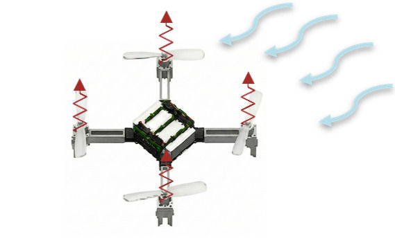
Drone Dynamics

We consider the drone system to have the following states: (p, v, q) for world frame position, velocity and orientation using quaternions. For simplification, the control input is assumed to be (f, Ω), for thrust force f and body angular velocity Ω, which is often found in commercial flight controllers. Then, the drone dynamics can be written as,

where ¯q (qbar but wix cannot render it) is the conjugate, e3 = [0, 0, 1]^T , (qe3 ¯q), (qΩ) are quaternion multiplications, m = 0.73, g = 9.81

Simulation

To simulate the given system, we use RK4 scheme for numerical integration. My implementation for the closed loop system with the controller can be written as

where dt = 10−4. This scheme works well with trajectories evolving on Euclidean spaces. Since our drone model uses unit quaternions, this scheme cannot ensure ˙q (qdot) dynamics will be followed correctly. For a more intuitive case, consider rotation matrix and an equation ˙R = f(R). If we were to perform numerical integration using some form of R = R + dtf(R), the addition cannot ensure R will remain a valid rotation matrix. This is because such addition is not defined on SO(3).

Feedback Integrators

We will use the theory of feedback integrators (or stable embedding) to fix this. Consider we extend rotation matrix R from SO(3) into R3×3 space but we put an additional constraint on its dynamics such that ∥R^T R − I∥ → 0. This will ensure the integration scheme works correctly while the constraint on R is still maintained (My explanation is not rigorous). This is easy to add to our system equations using an additional term −α(|q|2 − 1)q that ensures q ∈ S3:

The differences with using α = 0 and α̸ = 0 will be shown in the results section.

Trajectory

We generate a basic helical trajectory to be followed by the drone as,

where the following values are considered ω = π/5 , r = 5, h = 1. Please note that I am not performing optimal trajectory generation. I am only making an independent trajectory wrt time that can be followed by the controllers.

Controller 1: PD+P

We design a PD controller to track the position+velocity as,

To align the orientation with thrust vector Fd(t), compute the error in orientation as

which provides proportional control for unit quaternions q along S3. This gives us (f, Ω) control inputs.

Controller 2: Nonlinear control toolbox

For controller 2, I used a nonlinear control toolbox to directly solve for an optimal feedback controller as u = −K ∗ poly(x) (not meant for tracking per se). For my tests, I just vary the reference position using p_d with time. Although not perfect, this still works for few cases. However while solving for this controller, we need to consider a condition that wasn’t considered in the previous controller, i.e. f is not in R but instead f > 0 i.e. f in R_+. This was not considered before since the gravity compensation makes f positive most of the time. To fix this, we extend the dynamics as,

which forces thrust f to be positive and we have our control inputs as (u0, Ω). It is easy to see that on solving for f it gives f = f(0)*exp(integral u_0 dt) > 0. The cost Lagrangian is taken as L = x^T Qx + u^T Ru, with reference position and velocity to be [0, 0, 0]^T , orientation as [1, 0, 0, 0] and thrust as mg. Solving it gives us controller u(x) and for tracking I just consider u(x − pd).

Controller 3: Energy tank based passivity controller

The idea is to attach an energy tank between the controller and the robot so that if the controller acts in a non-passive way, the tank can be used to consume stored energy. Here the tank is a port-Hamiltonian system with ˙x(t) = 1/x_t*D(x) + u_t, y_t = x_t connected by a Dirac structure. The tank’s state x_t changes to ensure the non-passive energy from the controller is stored or extracted from the tank’s energy T = 1/2*x^2_t.

For more information you can check the paper: A. Pupa, P. R. Giordano and C. Secchi, “Optimal Energy Tank Initialization for Minimum Sensitivity to Model Uncertainties,” 2023 IEEE/RSJ International Conference on Intelligent Robots and Systems (IROS), Detroit, MI, USA, 2023, pp. 8192-8199

For controller 3, I tried to use some form of energy tank system as a dynamic feedback

controller to our system. Similar to controller 2, I introduce an extension to the system, which I believe is quite nonlinear. We consider a tank system with state ϵ < x_t < Tmax that evolves as ˙x_t = −α_2x_t + β(x_t) ω(u, y), where α_2 provides dissipation and β(x_t) = step(x_t < Tmax) goes to 0 when tank energy tries to go beyond limit. Our control inputs are now modified to follow this dynamic system’s behavior as umod = α_3(t)u, where α_3(t) = step(x_t > ϵ) which activates the control only if the energy of the tank is greater than the minimum threshold.

I was unable to find a valid ω(u, y) energy flow function and hence instead used a form of power, P = f v · qe3 ¯q + ∥Ω∥2 instead of uT y. For this task we just use the PD+P controller (controller 1) since we know this would be a passive system. Hence we have,

(Note: I might have made mistakes in forming a correct passive interconnection though). However, we can see from the equations that we have a system whose energy is regulated within a certain range. This didn’t work as expected however it was a learning experience.

Results

Controller 1 Tracking: MSE: 0.7, which works quite well for tracking tasks.

Controller 2 Tracking: MSE: 1.5, which is higher than controller 1, mainly because this one was not built for tracking.

Controller 3 Energy: The tank state xt varied as follows (1st figure). It followed exactly the same controller 1 behavior except that there was a tank system to force shutdown the system in certain cases when x_t > Tmax.

Stable Embedding: In the image above (2nd and 3rd figures), we can see how unit quaternion condition diverges without stable embedding (α = 0, blue) and stays within range with the technique (α = 1, red). Left figure is for controller 1 and right one is for controller 2.

Conclusion

Through this study, I examined drone dynamics, RK4 integration for simulation, the

effectiveness of feedback integrators, and positive thrust force constraint. The study ends with building two controllers for this system, using PD+P and nonlinear optimal control, the results of which are showed in the end.

– While the translational control is almost similar for both, the rotational control varies a lot between the two implementations.

– Another point to note is that the body thrust direction is not regulated in controller 2 unlike controller 1 where the orientation error between thrust force and current orientation (¯qqd) is fed back as error.

– For future work: Another thing to consider is the case of passive (PD, D) controllers and the non-passive nonlinear optimal feedback controller in the form of polynomial functions of x. There could also be more analysis on building passive controllers for such systems.