2024; Robot Control: Flexible Joint Robots

About the Project

I took a course called EE683: Robot Control by Professor Min Jun Kim at KAIST during my 2nd semester. One good thing about the course was the bi-weekly assignment which had one specific part where the students were free to implement any algorithm and provide simulation results. I ended up implementing a lot of the techniques and models learned in the course. These are a series of blog posts that cover some of those sections since I felt like it was worth sharing.

Note that all of these are implemented from scratch, with very few sections requiring MATLAB toolboxes. Also note that just because the specific part was in the report, it does not mean that it worked perfectly; given more time, I would've probably improved it, especially with regards to gain tuning for controllers.

All the work was done in MATLAB and the files will be shared soon on Github. If I have more time, I will also reexplain everything in simpler words.

You can download this full report here:

Flexible Joint Robots

Flexible joint robots are basically manipulators where the input torque to the joints first pass through a spring-link system between the motor and the actual joint making it "flexible". This makes it way more difficult to construct controllers and analyze the system since it becomes underactuated. Note that this is not flexible body robot.

We remember that our rigid joint robot can be modeled as (M (q) + N^2 B) ¨q + C(q, ˙q)˙q + g(q) = τ, where M (q) + N^2 B includes the link and motor inertia. In flexible joint robots this is not connected directly anymore and is instead passed through a spring system as

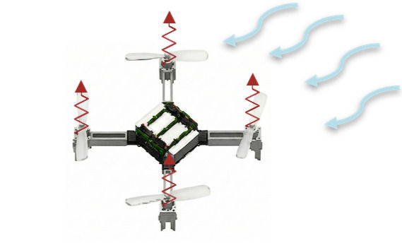
This is better visualized by the figure above where the motor and the link are separated through joint torque. The input torque provided to the motor causes motor rotation θ and generates the joint torque τ_j in the spring. This requires us to either measure the joint torque or the rotation on the link side through an encoder since motor rotation and link rotation are not the same anymore (θ /= q). For a simplified modelwith spring transfer, we can have τ_j = K_j (θ − q). One should note that the joint torque sensor (which uses an internal spring system for measurements) can also introduce flexibility by itself. There also exists inertial coupling between motors and the links, which can, however, be neglected in practice. These robots are also under-actuated, with increased states (θ, ˙θ, q, ˙q).

In this study, I tried to implement and simulate flexible joint robot dynamics. But I implemented it for a very simple system of a non-linear double pendulum. This helps me with simplifying the equations since I have massless links. I explain the process of the derivation and the use of MATLAB to derive everything in symbolic form. Then I implement the different control methods we learned in the lectures.

Finding M and C for nonlinear double pendulum

I took a double pendulum with link lengths l1, l2 and point mass m1, m2 attached to each end. The joint angle q1 is defined as the angle wrt vertical and q2 as the angle wrt previouslink. For such a system, we have the following inertia matrix written in symbolic form wrt variables q = [q1, q2]^T ([q1, q2] in MATLAB):

The Coriolis/centrifugal terms for this system can be calculated as C_ij = (∂M_ij/∂q)*˙q:

where the calculations have been represented here in compact form to save space. In MATLAB this is implemented using as jacobian(reshape(M,4,1), [q1, q2])*[q1dot, q2dot] for other symbolic variables [q1dot, q2dot]. Note that this is not the full C term and additional terms from kinetic energy is yet to be calculated. This was done to ensure easy code in MATLAB.

Modeling the system

We use Euler-Lagrange equations to find the system equations as

which is implemented in MATLAB as just qddot = inv(M)*(jacobian(L, [q1, q2])’ - C*[q1dot, q2dot] + u). We can easily see that this jacobian term will give the gravity compensation vector and the additional term from the kinetic energy which can be added to C term. Then our final system with state x = [q1, q2, ˙q1, ˙q2]^T is

Final rigid system

For masses 1kg and link lengths 1m each, the final symbolic matrices are

Making it flexible!

To induce flexible behavior, the system equations are now expanded to include a separate θ = [θ1, θ2]^T and ˙θ variables as ¨θ = B^{−1}(u − K_j (θ − q)). The τ_j = K_j (θ − q) term also replaces u from the original system equation. For this I had to use an ode15s stiff solver since my RK4 implementation was insufficient for it. In my simulation B = [1e-4, 0; 0, 1e-4] kgm2 and Kj = [1e5, 0; 0, 1e5] with very high stiffness. The overall state is 8 dimensional with 2 inputs now.

Controller1: PD+g controller

This is a PD controller with gravity compensation just implemented as u = K_P (q_d − q) + K_D (0 − ˙q) + g(q). This will be tested directly on both rigid and flexible joint robots

Controller2: Tomei controller

This is the controller from P. Tomei, “A simple PD controller for robots with elastic joints,” in IEEE Transactions on Automatic Control, vol. 36, no. 10, pp. 1208-1213, Oct. 1991, hereafter referred to as Tomei controller. We just have the reference wrt θ as θ_d = q_d + K^{-1}_j g(q_d) and u = K_P (θ_d − θ) + K_D (0 − ˙θ_d) + g(q_d).

Tomei controller comes from the idea that PD controller is sufficient to stabilize rigid manipulators and so a similar PD controller can also be employed for flexible joint manipulators. For more details please find the paper, the design of the matrices and reference θ_d is explained there.

Controller2: Inertia shaping controller

I find τ_j = K_j (θ − q), use a PD controller for unew = P D(q_d, q) and define the motor input as u = (1 − BB^{−1}_θ )τj + BB^{−1}_θ u_new with B_θ in the range 1e-6. I am tired of writing down the equations in wix without the possibility of rendering it, so for this controller please see this from my original report:

Results

All the gains are KP = [10, 0; 0, 10] and KD = [5, 0; 0, 5].

1. PD+gravity without flexible joint: For reference [π/2, π/2, 0, 0].

   

2. PD+gravity with flexible joint: For reference [π/2, π/2, 0, 0]. We can see the chattering in the velocities due to the flexible joint and hence takes a long time to converge to a solution.

   

3. Tomei controller with flexible joint: For reference [π/2, π/2, 0, 0]. There is no chattering and the results are quick. Note that I assumed the α condition is satisfied.

   

4. Inertia shaping controller: For reference [π/2, π/2, 0, 0]. Shows behavior similar to PD controller, maybe because I couldn’t tune the B_θ matrix correctly.

   

Conclusion

Nonlinear double pendulum system was implemented using symbolic equations in MATLAB and then simulated. This was extended to flexible joints. Different controllers were then implemented which showcased better performance with flexible joints especially the Tomei controller.